PyAFV

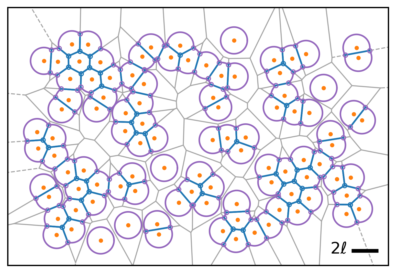
PyAFV is a Python package for simulating cellular tissues based on the 2D active finite Voronoi (AFV) model. It provides a computational framework for investigating collective cell behaviors such as motility, adhesion, jamming, and tissue fracture in active matter and biophysical systems. In contrast to standard vertex or Voronoi models, the AFV model incorporates finite interaction ranges and cell-medium interfaces, allowing for detachment, free boundaries, and fragmentation. The package includes tools for geometry handling, time evolution, and analysis of cell configurations. The AFV formalism was introduced and further developed in, for example, Refs. [1–3].

Installation

PyAFV is available on PyPI and can be installed using pip directly:

pip install pyafv

The package supports Python ≥ 3.10 and < 3.15, including Python 3.14t (the free-threaded, no-GIL build). To verify that the installation was successful and that the correct version is installed, run the following in Python:

import pyafv
print(pyafv.__version__)

As an alternative, you can install PyAFV via conda from the conda-forge channel:

conda install -c conda-forge pyafv

If you go this route, note that for Python 3.14 the conda-forge distribution currently provides only the GIL-enabled build.

See the documentation for instructions on installing the package from source or in offline environments.

Install using Docker 🐳

PyAFV can also be installed via containerized environments. Pull the Docker image from Docker Hub:

docker pull wwang721/pyafv:latest

The image is also available via the GitHub Container Registry (GHCR) under GitHub Packages; use ghcr.io/wwang721/pyafv to pull from GHCR instead.

Usage

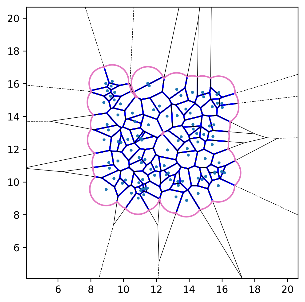
Here is a simple example to get you started, demonstrating how to construct a finite-Voronoi diagram (click the Google Colab badge above to run the notebook directly):

import numpy as np
import pyafv as afv

N = 100                                          # number of cells
pts = np.random.rand(N, 2) * 10                  # initial positions
params = afv.PhysicalParams(r=1.0)               # use default parameter values
sim = afv.FiniteVoronoiSimulator(pts, params)    # initialize the simulator
sim.plot_2d(show=True)                           # visualize the Voronoi diagram

To compute the conservative forces and extract detailed geometric information (e.g., cell areas, vertices, and edges), call:

diag = sim.build()

The returned object diag is a Python dict containing these quantities. Refer to the documentation for more detailed usage.

Simulation previews

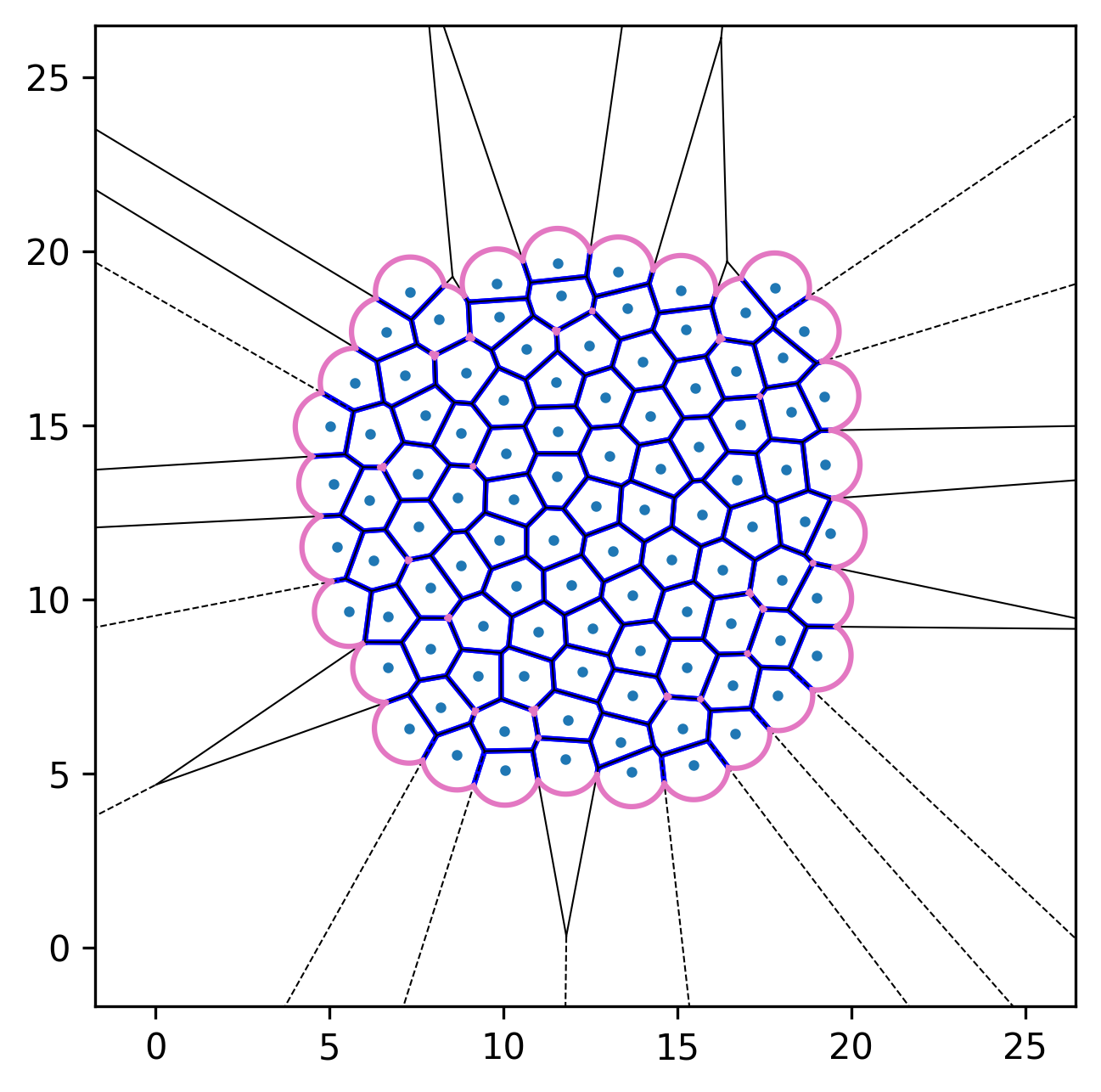
Below are representative simulation snapshots generated using the code:

Model illustration	Periodic boundary conditions

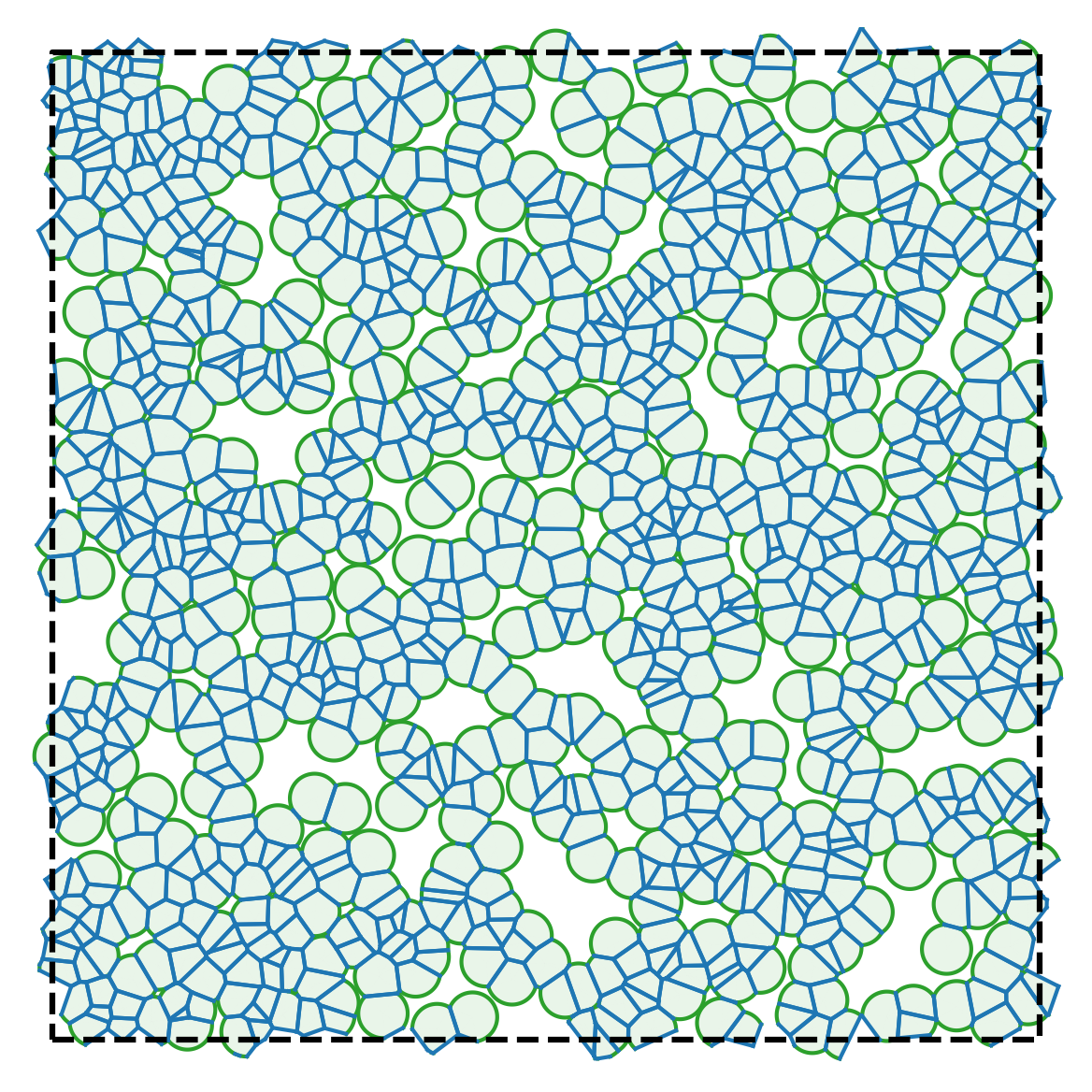Initial configuration	After relaxation	Active dynamics enabled

More information

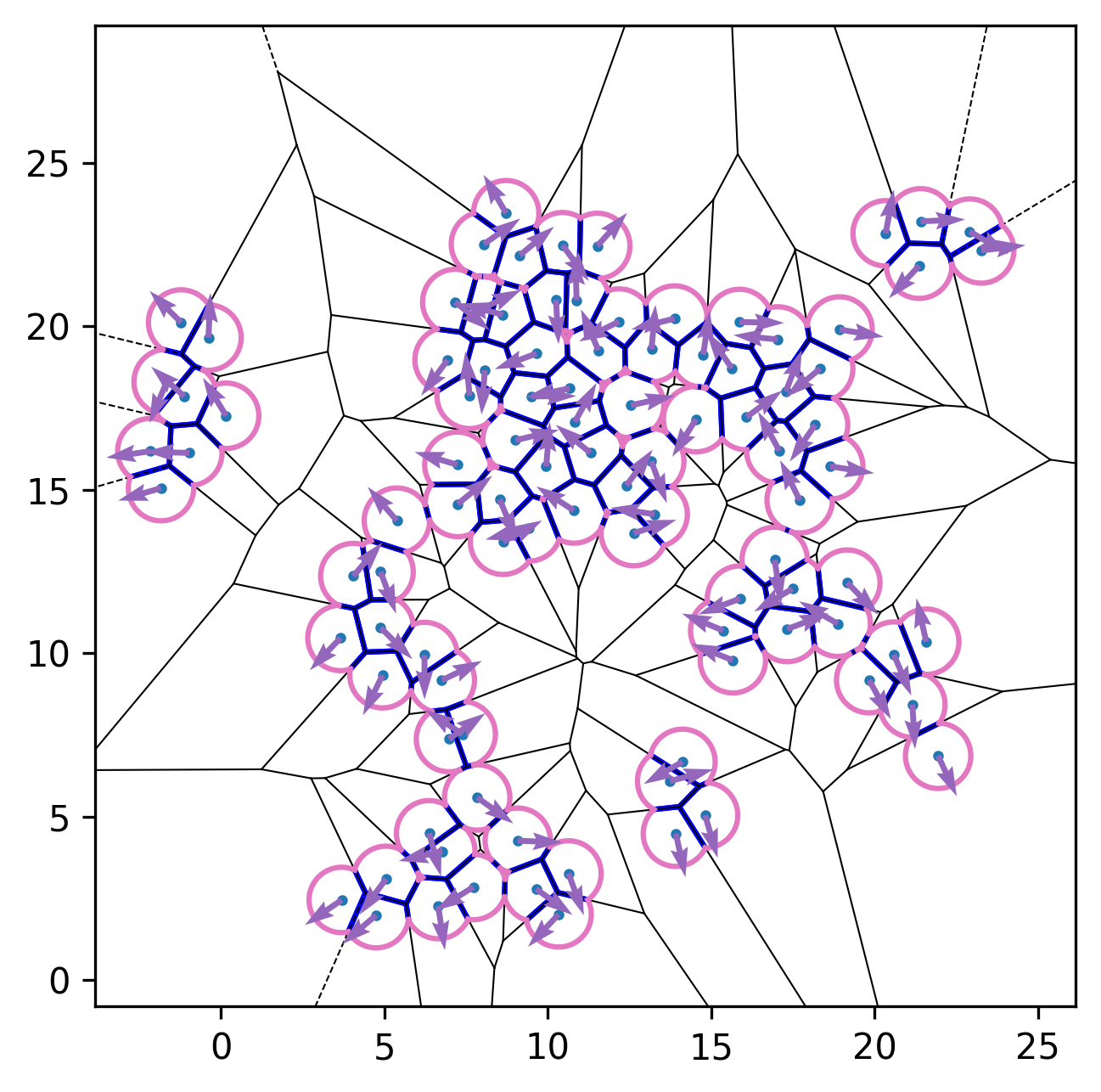• Full documentation on readthedocs or as a single PDF file.

• See CONTRIBUTING.md or the documentation for local development instructions.

• See some important issues for additional context, such as:

  • QhullError when 3+ points are collinear #1 [Closed - see comments]
  • Add customized plotting to examples illustrating access to vertices and edges #5 [Completed in PR #7]
  • Time step dependence of intercellular adhesion in simulations #8 [Closed in PR #9]

• Some releases of this repository are cross-listed on Zenodo:

  

References

[1]	J. Huang, H. Levine, and D. Bi, Bridging the gap between collective motility and epithelial-mesenchymal transitions through the active finite Voronoi model, Soft Matter 19, 9389 (2023).
[2]	E. Teomy, D. A. Kessler, and H. Levine, Confluent and nonconfluent phases in a model of cell tissue, Phys. Rev. E 98, 042418 (2018).
[3]	W. Wang (汪巍) and B. A. Camley, Divergence of detachment forces in the finite-Voronoi model, manuscript in preparation (2026).