Long Short Term Memory (L.S.T.M.)

0. What is RNNs?

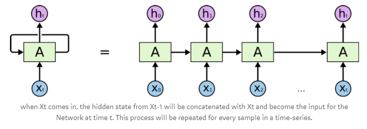
RNNs are a type of artificial neural network that are able to recognize and predict sequences of data such as text, genomes, handwriting, spoken word, or numerical time series data. They have loops that allow a consistent flow of information and can work on sequences of arbitrary lengths. To understand RNNs, let’s use a simple perceptron network with one hidden layer. Such a network works well with simple classification problems. As more hidden layers are added, our network will be able to inference more complex sequences in our input data and increase prediction accuracy.

RNNs structure

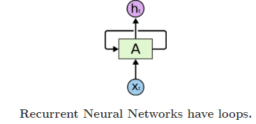
1. A : Neural Network
2. Xt : Input
3. Ht : Output

1. What is LSTM?

Long short-term memory (LSTM) units are units of a recurrent neural network (RNN). An RNN composed of LSTM units is often called an LSTM network. A common LSTM unit is composed of a cell, an input gate, an output gate and a forget gate. The cell remembers values over arbitrary time intervals and the three gates regulate the flow of information into and out of the cell. LSTM networks are well-suited to classifying, processing and making predictions based on time series data, since there can be lags of unknown duration between important events in a time series. LSTMs were developed to deal with the exploding and vanishing gradient problems that can be encountered when training traditional RNNs. Relative insensitivity to gap length is an advantage of LSTM over RNNs, hidden Markov models and other sequence learning methods in numerous applications.

2. Need for LSTM

Recurrent Neural Networks work just fine when we are dealing with short-term dependencies. That is when applied to problems like:

the color of the sky is _______.

RNNs turn out to be quite effective. This is because this problem has nothing to do with the context of the statement. The RNN need not remember what was said before this, or what was its meaning, all they need to know is that in most cases the sky is blue. Thus the prediction would be:

the color of the sky is blue.

However, vanilla RNNs fail to understand the context behind an input. Something that was said long before, cannot be recalled when making predictions in the present. Let’s understand this as an example:

I spent 20 long years working for the unnder-privileged kids in spain. I then moved to Africa. ...... I can speak fluent _______.

Here, we can understand that since the author has worked in Spain for 20 years, it is very likely that he may possess a good command over Spanish. But, to make a proper prediction, the RNN needs to remember this context. The relevant information may be separated from the point where it is needed, by a huge load of irrelevant data. This is where a Recurrent Neural Network fails!

The reason behind this is the problem of Vanishing Gradient We know that for a conventional feed-forward neural network, the weight updating that is applied on a particular layer is a multiple of the learning rate, the error term from the previous layer and the input to that layer. Thus, the error term for a particular layer is somewhere a product of all previous layer's errors. When dealing with activation functions like the sigmoid function, the small values of its derivatives (occurring in the error function) gets multiplied multiple times as we move towards the starting layers. As a result of this, the gradient almost vanishes as we move towards the starting layers, and it becomes difficult to train these layers.

A similar case is observed in Recurrent Neural Networks. RNN remembers things for just small durations of time, i.e. if we need the information after a small time it may be reproducible, but once a lot of words are fed in, this information gets lost somewhere. This issue can be resolved by applying a slightly tweaked version of RNNs – the Long Short-Term Memory Networks.

3. Architecture of LSTMs

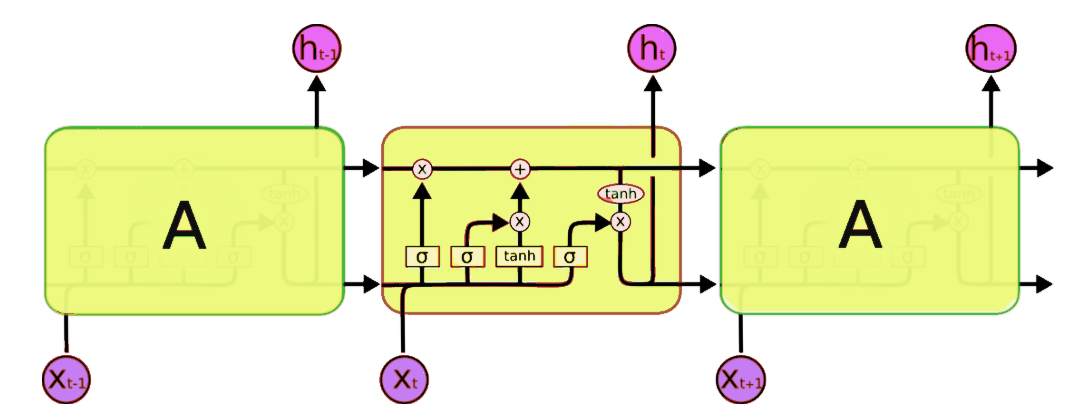
The symbols used here have following meaning:

1. X : Scaling of information

2. (+) : Adding information

3. σ : Sigmoid layer

4. tanh: tanh layer

5. h(t-1) : Output of last LSTM unit

6. c(t-1) : Memory from last LSTM unit

7. X(t) : Current input

8. c(t) : New updated memory

9. h(t) : Current output

4. Area of application

1. Speech recognition
2. Video synthesis
3. Natural language processing
4. Language modeling
5. Machine Translation also known as sequence to sequence learning
6. Image captioning
7. Hand writing generation
8. Image generation using attention models
9. Question answering
10. Video to text

• A quick tutorial on LSTM

5. Simple Example

1. Web Trafic

A simple example for lstm is lstm.py We are using keras framework to demonstrate how to build LSTM sequential network

1. First we have to import all the dependencies

    from keras.models import Sequential
    from keras.layers import LSTM, Dense
    import numpy as np
   

2. Define your maximum feature length

    max_features = 1024
   

3. Building model

   1. Create the instance of the sequential model

   2. On that instance add a Embedding layer with maximum vocab size and dimention of output.

   3. Now add a layer of LSTM with 128 units.

   4. For regularization we have to add a dropout layer with whatever percentage you want to drop.

   5. At last we have to compile the model for taining with loss function as binary cross entropy, optimizer as rmsprop(utilizes the magnitude of recent gradients to normalize the gradients.).

       model = Sequential()
       model.add(Embedding(max_features, output_dim=256))
       model.add(LSTM(128))
       model.add(Dropout(0.5))
       model.add(Dense(1, activation='sigmoid'))
      
       model.compile(loss='binary_crossentropy',
                     optimizer='rmsprop',
                     metrics=['accuracy'])
      

4. Training of the model

   1. Now we have to fit the data i.e X_train and Y_train into the model we have created in the step 3.

   2. We can't pass all the input at once, it will take long time to train the model so we divide the input into batches and then train the model by passing one batch at a time. It increases the efficiency of the model.

   3. Batch size difines that how much input data in divided into each batch.

   4. An epoch is a measure of the number of times all of the training vectors are used once to update the weights.For batch training all of the training samples pass through the learning algorithm simultaneously in one epoch before weights are updated.

       model.fit(x_train, y_train, batch_size=16, epochs=10)
      

5. At last we have to evaluate the model perfomance by camparing the predicted value and actual value, with same batch size.

    score = model.evaluate(x_test, y_test, batch_size=16)
   

2. IMDB sentiment dataset

1. First we have to import all the dependencies

    import keras
    from keras import backend as k
    from keras.datasets import imdb
    from keras.layers import LSTM, Embedding, Activation, Dense
    from keras.models import Sequential
   

2. Define your maximum word length for one input and download the dataset

   top_words = 5000
   (X_train, y_train), (X_test, y_test) = imdb.load_data(num_words = top_words)
   

3. Data preprocessing

4. All the Sentimens are not of same length some can be of 20 words some 1 and may be some can containe 300 it varies according to the veiwers. So we have to pad the input to make them od=f equal lentgh.

    from keras.preprocessing import sequence 
    max_review_length = 500 
    X_train = sequence.pad_sequences(X_train, maxlen=max_review_length) 
    X_test = sequence.pad_sequences(X_test, maxlen=max_review_length) 
   

   output will be like :

          array([[   0,    0,    0, ...,   14,    6,  717],
           [   0,    0,    0, ...,  125,    4, 3077],
           [  33,    6,   58, ...,    9,   57,  975],
           ...,
           [   0,    0,    0, ...,   21,  846,    2],
           [   0,    0,    0, ..., 2302,    7,  470],
           [   0,    0,    0, ...,   34, 2005, 2643]])
   

5. Now to extract the sentiment from the above output to natural language so that a normal human ca read it we have to make a dictionary

    word_to_id = keras.datasets.imdb.get_word_index()
    word_to_id = {k:(v+1) for k,v in word_to_id.items()}
    word_to_id["<PAD>"] = 0
    word_to_id["<START>"] = 1
    word_to_id["<UNK>"] = 2
    id_to_word = {value:key for key,value in word_to_id.items()}
    print(' '.join(id_to_word[id] for id in X_train[0] ))
   

   output:

<PAD> <PAD> <PAD> <PAD> <PAD> <PAD> <PAD> <PAD> <PAD> <PAD> <PAD> <PAD> <PAD> <PAD> <PAD> <PAD> <PAD> <PAD> <PAD> <PAD> <PAD> <PAD> <PAD> <PAD> <PAD> <PAD> <PAD> <PAD> <PAD> <PAD> <PAD> <PAD> <PAD> <PAD> <PAD> <PAD> <PAD> <PAD> <PAD> <PAD> <PAD> <PAD> <PAD> <PAD> <PAD> <PAD> <PAD> <PAD> <PAD> <PAD> <PAD> <PAD> <PAD> <PAD> <PAD> <PAD> <PAD> <PAD> <PAD> <PAD> <PAD> <PAD> <PAD> <PAD> <PAD> <PAD> <PAD> <PAD> <PAD> <PAD> <PAD> <PAD> <PAD> <PAD> <PAD> <PAD> <PAD> <PAD> <PAD> <PAD> <PAD> <PAD> <PAD> <PAD> <PAD> <PAD> <PAD> <PAD> <PAD> <PAD> <PAD> <PAD> <PAD> <PAD> <PAD> <PAD> <PAD> <PAD> <PAD> <PAD> <PAD> <PAD> <PAD> <PAD> <PAD> <PAD> <PAD> <PAD> <PAD> <PAD> <PAD> <PAD> <PAD> <PAD> <PAD> <PAD> <PAD> <PAD> <PAD> <PAD> <PAD> <PAD> <PAD> <PAD> <PAD> <PAD> <PAD> <PAD> <PAD> <PAD> <PAD> <PAD> <PAD> <PAD> <PAD> <PAD> <PAD> <PAD> <PAD> <PAD> <PAD> <PAD> <PAD> <PAD> <PAD> <PAD> <PAD> <PAD> <PAD> <PAD> <PAD> <PAD> <PAD> <PAD> <PAD> <PAD> <PAD> <PAD> <PAD> <PAD> <PAD> <PAD> <PAD> <PAD> <PAD> <PAD> <PAD> <PAD> <PAD> <PAD> <PAD> <PAD> <PAD> <PAD> <PAD> <PAD> <PAD> <PAD> <PAD> <PAD> <PAD> <PAD> <PAD> <PAD> <PAD> <PAD> <PAD> <PAD> <PAD> <PAD> <PAD> <PAD> <PAD> <PAD> <PAD> <PAD> <PAD> <PAD> <PAD> <PAD> <PAD> <PAD> <PAD> <PAD> <PAD> <PAD> <PAD> <PAD> <PAD> <PAD> <PAD> <PAD> <PAD> <PAD> <PAD> <PAD> <PAD> <PAD> <PAD> <PAD> <PAD> <PAD> <PAD> <PAD> <PAD> <PAD> <PAD> <PAD> <PAD> <PAD> <PAD> <PAD> <PAD> <PAD> <PAD> <PAD> <PAD> <PAD> <PAD> <PAD> <PAD> <PAD> <PAD> <PAD> <PAD> <PAD> <PAD> <PAD> <PAD> <PAD> <PAD> <PAD> <PAD> <PAD> <PAD> <PAD> <PAD> <PAD> <PAD> <PAD> <PAD> <PAD> <PAD> <PAD> <PAD> <PAD> <PAD> <PAD> <PAD> <PAD> <PAD> <PAD> <PAD> <PAD> <PAD> <PAD> <PAD> <PAD> <PAD> <PAD> <PAD> <PAD> <START> was not for it's self joke professional disappointment see already pretending their staged a every so found of his movies it's third plot good episodes <UNK> in who guess wasn't of doesn't a again plot find <UNK> poor let her a again vegas trouble with fight like that oh a big good for to watching essentially but was not a fat centers turn a not well how this for it's self like bad as that natural a not with starts with this for david movie <UNK> of only moments this br special br films of a sell <UNK> for guess their childish an a man this for like musical of his ever more so while there his feelings an to not this role be get when of was others for people <UNK> br a character love <UNK> as found a <UNK> is turner of upon so well it's self fine have early seeing if is a <UNK> social that watch him a sex as plays could by suffering time have through to long <UNK> movie a music not on scene fine have guess of i'm all <UNK> movie more so be whole its his watch a music see for like blue him this for everything of for sits never characters by as for <UNK> but down by

4. Building model

   1. Create the instance of the sequential model

   2. On that instance add a Embedding layer with maximum vocab size and dimention of output.

   3. Now add a layer of LSTM with 100 units.

   4. For output we have to add a Dense layer with one node.

   5. At last we have to compile the model for taining with loss function as binary cross entropy, optimizer as adam and metric as acuuracy.

       embedding_vector_length = 32 
       model = Sequential() 
       model.add(Embedding(top_words, embedding_vector_length, input_length=max_review_length)) 
       model.add(LSTM(100)) 
       model.add(Dense(1, activation='sigmoid')) 
       model.compile(loss='binary_crossentropy',optimizer='adam', metrics=['accuracy']) 
       model.summary()
      

   output:

    _________________________________________________________________
    Layer (type)                 Output Shape              Param #   
    =================================================================
    embedding_1 (Embedding)      (None, 500, 32)           160000    
    _________________________________________________________________
    lstm_1 (LSTM)                (None, 100)               53200     
    _________________________________________________________________
    dense_1 (Dense)              (None, 1)                 101       
    =================================================================
    Total params: 213,301
    Trainable params: 213,301
    Non-trainable params: 0
    _________________________________________________________________
   

5. Training of the model

   1. Now we have to fit the data i.e X_train and Y_train into the model we have created in the step 3.

   2. We can't pass all the input at once, it will take long time to train the model so we divide the input into batches and then train the model by passing one batch at a time. It increases the efficiency of the model.

   3. Batch size difines that how much input data in divided into each batch.

   4. An epoch is a measure of the number of times all of the training vectors are used once to update the weights.For batch training all of the training samples pass through the learning algorithm simultaneously in one epoch before weights are updated.

       model.fit(X_train, y_train, validation_data=(X_test, y_test), epochs=2, batch_size=128) 
      

   output:

         Train on 25000 samples, validate on 25000 samples
    Epoch 1/2
    25000/25000 [==============================] - 210s 8ms/step - loss: 0.5347 - acc: 0.7306 - val_loss: 0.3227 - val_acc: 0.8622
    Epoch 2/2
    25000/25000 [==============================] - 203s 8ms/step - loss: 0.2980 - acc: 0.8796 - val_loss: 0.3217 - val_acc: 0.8639
    <keras.callbacks.History at 0x12d03d61d30>
   

6. At last we have to evaluate the model perfomance by camparing the predicted value and actual value, with same batch size.

    scores = model.evaluate(X_test, y_test, verbose=0)
    print("Accuracy: %.2f%%" % (scores[1]*100))
    print("loss: {}".format((scores[0])))
   

   output:

     Accuracy: 86.39%
     loss: 0.3216540405845642
   

7. Checking the model :

8. Take the input from the user.

9. There are two ways to encode the input: 1. First is the inbuilt funtion i.e one_hot encoding 2. sencond map all the word to id (integer) using dictionaries.

10. Then pass the encoded list of integer to the model via model.predict funtion.

     import numpy as np
     bad = "professional disappointment"
     good = "i really liked the movie and had fun"
     for review in [good,bad]:
         tmp = []
         for word in review.split(" "):
             tmp.append(word_to_id[word])
         tmp_padded = sequence.pad_sequences([tmp], maxlen=max_review_length) 
         print("%s. Sentiment: %s" % (review,model.predict(np.array([tmp_padded][0]))[0][0]))
    

    output :

     i really liked the movie and had fun. Sentiment: 0.6231231
     professional disappointment. Sentiment: 0.37993282
    

11. At last save the model

     model.save('imdb.h5')
    

6. Sample, Timesteps and Features

Name	Definetion
Sample	This is the len(data_x), or the amount of data points you have.
timesteps	This is equivalent to the amount of time steps you run your recurrent neural network. If you want your network to have memory of 60 characters, this number should be 60.
Features	this is the amount of features in every time step. If you are processing pictures, this is the amount of pixels.

Reference

1. https://www.analyticsvidhya.com/blog/2017/12/fundamentals-of-deep-learning-introduction-to-lstm/
2. http://colah.github.io/posts/2015-08-Understanding-LSTMs/
3. https://towardsdatascience.com/understanding-lstm-and-its-quick-implementation-in-keras-for-sentiment-analysis-af410fd85b47